Linear Regression Made Simple
The Basic Mathematics Behind Machine Learning
Many people, especially those new to the field, often show great interest in the field of machine learning, but shy away from the mathematics that govern it. I hope to demystify it for you by explaining, in simple terms, the math behind machine learning. Linear regression is one the most fundamental mathematical algorithms used in supervised learning.
You may ask, “What is linear regression?”
Regression, in English, means a return to a less developed state. The technical definition doesn’t stray far. Regression is a method of analysis used to understand the relationship between two or more variables. This is a valuable tool in prediction and optimization.
Let’s start understanding the principles behind linear regression, and gradient descent, graphically.

Simple Linear Regression
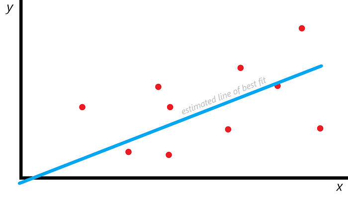
Let us assume, arbitrarily, we have a distribution of points as shown:

Linear regression seeks out an approximation of this distribution — a line that best explains the given distribution, a line that best describes the pattern of the data. Let us call this the best fit line. Intuitively, linear regression explains this exact thing.

We can algebraically represent the above line as y = h(x), where:
h(x) = θ₀ + θ₁ x
h stands for hypothesis, θ represents parameter, and x is a feature. The objective of performing linear regression on the data set is to find the optimum values of θ₀ and θ₁ such that h(x) is most suitable to explain the behavior of the data.
Above, we saw what is called simple linear regression, which involves only one explanatory variable. This method of linear regression has its use cases, but more often than not, we find ourselves needing to analyse more than one feature. This leads us to multiple linear regression.
Multiple Linear Regression
Multiple linear regression is similar to simple linear regression, with the additional complexity of taking into consideration n different features, as opposed to just one. The equation for the best fit line (hypothesis function) now looks like this:
h(x) = θ₀ + θ₁ x₁ + θ₂ x₂ + θ₃ x₃ + … + θₙ xₙ
The θ terms represent parameters, also called weights, and it is quite easy to understand why. From the equation of h(x), it is clear that the parameters determine the extent of influence of the features on the behavior of the system. We could also say θᵢ defines the importance of a particular feature xᵢ in the final output.
To better understand how we would apply multiple linear regression in the real world, let us take the famous example of the house pricing algorithm. Here, we use the features of the house (number of bedrooms, number of bathrooms, area, and location) to determine the price of a house. We could take other features into account as well, but for the sake of this example, let’s take these four.
Using our equation for the line of best fit on the first house, we have:
30 = θ₀ + 1 . θ₁ + 1 . θ₂ + 500 . θ₃ + 3 . θ₄
Similarly, we can create an equation for all the houses and hence find the optimal parameters.
Loss Function
Let us, for the sake of simplicity, assume a system of only one explanatory variable. A system of two variables would require us to draw a 2-d plane, and three explanatory variables would require a hyperplane to represent it. A hyperplane is impossible to visualize, so let’s stick to one explanatory variable.

We can clearly see our approximate best fit line is quite far from many of the points. Let’s call the vertical deviation of a point from the best fit line e. This e is the difference between predicted and actual values. Then, our goal is to minimize Σe. To do this, let us introduce a function:
J(θ) = Σe
J(θ) is called loss function, or error function. To further analyse and minimize the loss function, let’s expand e.
e is equal to the vertical distance between the actual point and a point on the estimated line of best fit. Since we do not want the distances to cancel out when we take its summation, we square this value.
e₁ = (h(x₁) - y₁)² , e₂ = (h(x₂) - y₂)² and so on…
Therefore, we have:
J(θ) = (1/2m) Σ(h(xᵢ) - yᵢ)², where i goes from 0 to m, m is the total number of examples.
The reason we take 1/m is because our summation value will be unnecessarily large otherwise, and we take 1/2 to help simplify computation, as you will see later. This is how we arrive at the loss function. This method of calculating error is called mean squared error.
Extrapolating our loss function to account for multiple additional dimensions, we have:
J(θ) = (1/2m) Σ(θ₀ + θ₁ x₁ᵢ + θ₂ x₂ᵢ + θ₃ x₃ᵢ + … + θₙ xₙᵢ - yᵢ)², i: 0 ➡ m
To find the optimal parameters, we employ a method known as gradient descent.
Finding the Slope at a Point on the Curve
To use gradient descent to find the optimal parameters, we need to know how to find the slope at each point on the curve. To understand this process graphically, let us again assume a case of simple linear regression, where h(x) = θ₀ + θ₁ x.
J(θ) = (1/2m) Σ(θ₀ + θ₁ x₁ᵢ - yᵢ)², i: 0 ➡ m
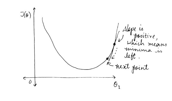
From the equation for J(θ), we can tell the plot between J(θ) and θ₁ will be that of a parabola, since the equation of a parabola is y = ax² + bx + c.

Once again, it is clear why I chose to graphically represent only a case of simple linear regression, as anything more would have required beyond three dimensions.
It becomes apparent that to minimize J(θ), we must find the local minima of the curve. Using basic calculus, to find the slope of the tangent at a particular point of a curve, we must differentiate the function and substitute the values corresponding to that particular point. Applying that knowledge here, using partial derivatives since J(θ) is a function of both θ₀ and θ₁, we get:
∂J(θ) / ∂θ₀ = (1/2m) 2 Σ(θ₀ + θ₁ x₁ᵢ - yᵢ)(1 + 0 – 0), i: 0 ➡ m
∂J(θ) / ∂θ₀ = (1/m) Σ(θ₀ + θ₁ x₁ᵢ - yᵢ), i: 0 ➡ m
∂J(θ) / ∂θ₀ = (1/m) Σ(h(xᵢ) - yᵢ), i: 0 ➡ m
Now we understand why I introduced a 2 in the denominator while defining the loss function.
Partially differentiating J(θ) with respect to θ₁, we get:
∂J(θ) / ∂θ₁ = (1/2m) 2 Σ(θ₀ + θ₁ x₁ᵢ - yᵢ)(0 + x₁ᵢ - 0), i: 0 ➡ m
∂J(θ) / ∂θ₁ = (1/m) Σ(θ₀ + θ₁ x₁ᵢ - yᵢ)(x₁ᵢ), i: 0 ➡ m
∂J(θ) / ∂θ₁ = (1/m) Σ(h(xᵢ) - yᵢ)(x₁ᵢ), i: 0 ➡ m
We can introduce a feature x₀ to h(x), where x₀ = 1.
h(x) = θ₀ x₀ + θ₁ x₁ + θ₂ x₂ + θ₃ x₃ + … + θₙ xₙ, where x₀ = 1
Then we can rewrite ∂J(θ)/∂θ₀ as:
∂J(θ) / ∂θ₀ = (1/m) Σ(h(xᵢ) - yᵢ)(x₀ᵢ), i: 0 ➡ m
Observing ∂J(θ)/∂θ₀ and ∂J(θ)/∂θ₁, we can make the generalization:
∂J(θ) / ∂θₙ = (1/m) Σ(h(xᵢ) - yᵢ)(xₙᵢ), i: 0 ➡ m
This is how we calculate the slope of the tangent at a point on the curve.
Gradient Descent
Gradient descent is an iterative optimization algorithm to find the local minima of a function. Let’s understand it in a step by step visualization.
Let us choose an arbitrary point on the curve, and find the slope of the tangent at that point. We already have the equation for it, above. The slope at that point tells us about which direction the minima is.
The minima is the point at which the value of J(θ) is minimum, which means at this point we will find our optimal parameter values.
If the slope at this point is negative, for instance, this tells us the minima is towards the right, and if the slope is positive, the minima is towards the left. In other words, the slope of the tangent points us towards the local minima.

Theoretically, now that we know which way to move, by iterating in incremental steps in the right direction, we must eventually come close to the optimal solution.
Now you may ask, “How do we know by how much we must move every iteration?”
This brings us to the final topic for this article, the learning rate.
Learning Rate
Gradient descent uses a hyperparameter called learning rate, α, to control the size of each step we take towards the optimal solution. A learning rate too small would result in too many required epochs to reach the optimal solution, and learning rate too large would risk overshooting the minima and diverging.
The perfect α will start comparatively high, and become successively smaller as we approach the minima, so as to find the perfect balance between number of epochs and precision. This can be done by having an α proportional to the slope at the point. The larger the slope, the larger the step we take in the minima’s direction.

Mathematically, we incorporate learning rate into our approach towards the minima as follows:
θₙ := θₙ - α (∂J(θₙ)/ ∂θₙ), or
θₙ := θₙ - α (slope)
Gradient Descent Optimizations
One of the problems with the concept of gradient descent arises when the error function doesn’t resemble a parabola and has multiple minimas. In this case, we always want to find the global minima of the function.
Gradient descent poses the risk of getting stuck in a local minima, depending on where we randomly initialise our weight (from where we start the gradient descent process).
One of the solutions to this would be running the algorithm several times with different initialised weights, hoping that one of these times, the minima found is global.
Another solution is by using Momentum, which is an optimization of gradient descent which can be visualised as us pushing the ball down a hill (the function). By principle, the ball would roll past local minima (assuming it starts at a high enough point) and if we incorporate air resistance the ball will eventually end up at the global minima.
If you read all the way, and found this useful, thanks! Feel free to leave suggestions or comments.

